 traj
traj
- Home
- FAQ
- Screenshots
- Features
- Documentation
- sourceforge project page.
- Download
- Acknowledgments
- CVS
- License
- stuff
- To Do/Wish List
A number of screenshots are given below. The description for each image appears above the image.
Initial view of the approximation for the equation of a spiral.
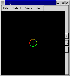
View of spiral after rotating it slightly.

View of spiral after rotating a little more..
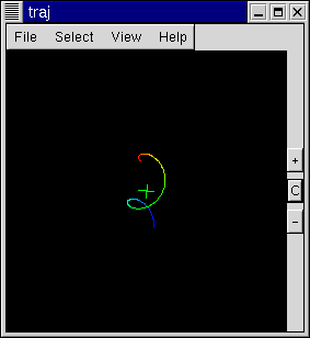
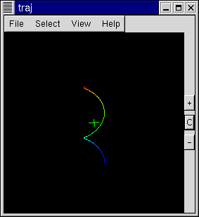
View of spiral after rotating a little more. This is close to a side view.
A view of the Lorenz attractor from straight down the z-axis.

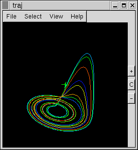
A side view of the Lorenz attractor after rotating it.
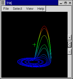
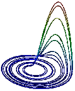
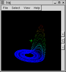
A view of the Lorenz attractro. Here the trajectory is colored by the time vairable. Red is smallest in time with purple the latest in time.
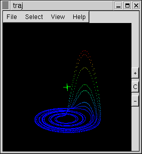
Another view of the Lorenz attractor. Instead of a solid line it is plotted as a dotted line.
Two plots at once. The spiral and the Lorenz attractor are plotted together.

Same as above, only they are both selected to be edited.
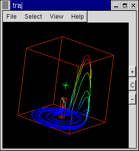
Same as above, except that only the spiral is selected.
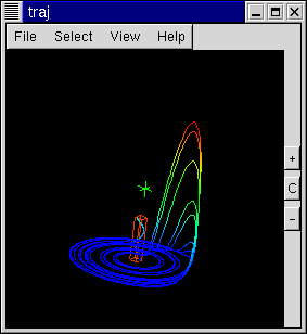
Same as above, except that only the Lorenz attractor is selected.
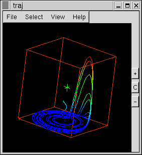
The main window with no trajectories plotted. This is the initial view upon start up.
A plot of the trajectory of the butterfly attractor. The trajectory is plotted as a dotted line.
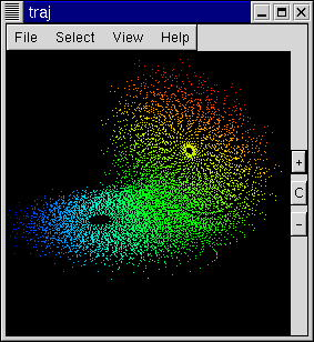
The Lorenz attractor. Again, it is plotted as dotted lines.
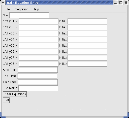
The dialog used to enter equations. This is a blank dialog with no equations entered.
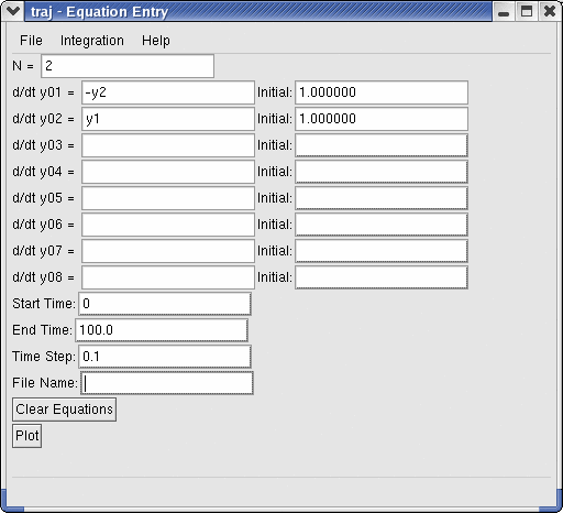
The equation window again, but now the differential equation for a spiral has been entered.
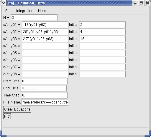
The equation window with the Lorenz equation entered.
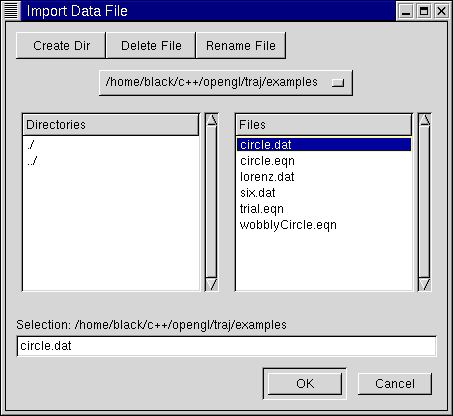
The file dialog. This is the standard gtk dialog used to open a data file. The program can save equations or it can read raw data files (text) for plotting.
The different axis can be set to whichever variable you would like in your phase space.
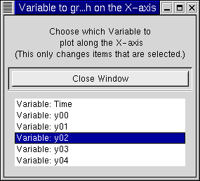
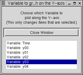
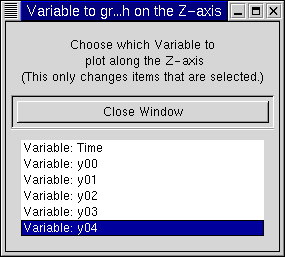
|
This project made possible through the generous support of sourceforge. |
|
This site hosted on cyclismo.org. |